Python interface#
For this tutorial, we will use the test data that can be downloaded from our git repository using the following commands.
git clone --filter=blob:none --no-checkout https://github.com/JaGeo/LobsterPy.git
cd LobsterPy
git sparse-checkout set tests/test_data
git read-tree -mu HEAD
Usage of Analysis, Description class and automatic plotting#
Basic usage : Analysis, Description#
Lets first import the necessary modules
from pathlib import Path

from pexpect.replwrap import python

from lobsterpy.cohp.analyze import Analysis
from lobsterpy.cohp.describe import Description
import warnings
warnings.filterwarnings('ignore')
#### Change directory to your Lobster computations (Change this cell block type to Code and remove formatting when executing locally)
directory = Path("LobsterPy") / "tests" / "test_data" / "CdF_comp_range"
# Initialize Analysis object
analyse = Analysis(
    path_to_poscar=directory / "CONTCAR.gz",
    path_to_icohplist=directory / "ICOHPLIST.lobster.gz",
    path_to_cohpcar=directory / "COHPCAR.lobster.gz",
    path_to_charge=directory / "CHARGE.lobster.gz",
    which_bonds="cation-anion",
)
# Initialize Description object and to get text description of the analysis
describe = Description(analysis_object=analyse)
describe.write_description()
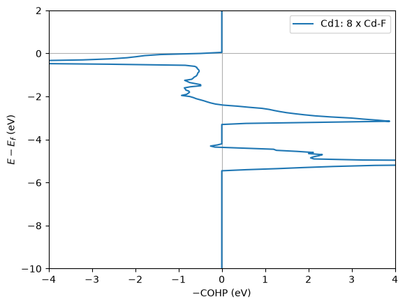
The compound CdF2 has 1 symmetry-independent cation(s) with relevant cation-anion interactions: Cd1.
Cd1 has a cubic (CN=8) coordination environment. It has 8 Cd-F (mean ICOHP: -0.62 eV, 26.944 percent antibonding interaction below EFermi) bonds.
# Get static plots for detected relevant bonds
describe.plot_cohps(ylim=[-10, 2], xlim=[-4, 4])
# Get interactive plots of relevant bonds,

# Setting label_resolved arg to True will plot each COHP curve separately, alongside summed COHP for the bonds.
fig = describe.plot_interactive_cohps(label_resolved=True, hide=True)
fig.show(renderer='notebook')
Due to sphinx rendering limitations for Plotly figures, the output is not directly visible within the notebook; please use the link to see the interactive label resolved plot
# Dict summarizing the automatic analysis results
analyse.condensed_bonding_analysis
{'formula': 'CdF2',
 'max_considered_bond_length': 5.98538,
 'limit_icohp': (-inf, -0.1),
 'number_of_considered_ions': 1,
 'sites': {0: {'env': 'C:8',
   'bonds': {'F': {'ICOHP_mean': '-0.62',
     'ICOHP_sum': '-4.97',
     'has_antibdg_states_below_Efermi': True,
     'number_of_bonds': 8,
     'bonding': {'integral': np.float64(7.89), 'perc': np.float64(0.73056)},
     'antibonding': {'integral': np.float64(2.91),
      'perc': np.float64(0.26944)}}},
   'ion': 'Cd',
   'charge': 1.57,
   'relevant_bonds': ['40', '33', '63', '30', '60', '53', '29', '64']}},
 'type_charges': 'Mulliken'}
# Dict with bonds identified
analyse.final_dict_bonds
{'Cd-F': {'ICOHP_mean': -0.62125, 'has_antbdg': True}}
# Dict with ions and their co-ordination environments
analyse.final_dict_ions
{'Cd': {'C:8': 1}}
Note
You can also perform automatic analysis using COBICAR(ICOBILIST.lobster) or COOPCAR(ICOOPLIST.lobster). You would need to set are_cobis/are_coops to True depending on the type of file you decide to analyze when you initialize the Analysis object. Change the default noise_cutoff value to 0.001 or lower, as ICOOP and ICOBI typically have smaller values and different units than ICOHP. Below is an example code snippet.
analyse = Analysis(
    path_to_poscar=directory / "CONTCAR.gz",
    path_to_icohplist=directory / "ICOBILIST.lobster.gz",
    path_to_cohpcar=directory / "COBICAR.lobster.gz",
    path_to_charge=directory / "CHARGE.lobster.gz",
    which_bonds="cation-anion",
    are_cobis=True,
    noise_cutoff=0.001,
)
Accessing other results is the same as the above.
Advanced usage : Analysis, Description#
LobsterPy now also allows for automatic orbital-wise analysis and plotting of COHPs, COBIs, and COOPs. To switch on orbital-wise analysis, one must set orbital_resolved arg to True. By default, orbitals contributing 5% or more relative to summed ICOHPs are considered in the analysis. One can change this default threshold using the orbital_cutoff argument. Here, we will set this cutoff value to 3%.
analyse = Analysis(
    path_to_poscar=directory / "CONTCAR.gz",
    path_to_icohplist=directory / "ICOHPLIST.lobster.gz",
    path_to_cohpcar=directory / "COHPCAR.lobster.gz",
    path_to_charge=directory / "CHARGE.lobster.gz",
    which_bonds="cation-anion",
    orbital_resolved=True,
    orbital_cutoff=0.03,
)
# Access the dict summarizing the results including orbital-wise analysis data
analyse.condensed_bonding_analysis
{'formula': 'CdF2',
 'max_considered_bond_length': 5.98538,
 'limit_icohp': (-inf, -0.1),
 'number_of_considered_ions': 1,
 'sites': {0: {'env': 'C:8',
   'bonds': {'F': {'ICOHP_mean': '-0.62',
     'ICOHP_sum': '-4.97',
     'has_antibdg_states_below_Efermi': True,
     'number_of_bonds': 8,
     'bonding': {'integral': np.float64(7.89), 'perc': np.float64(0.73056)},
     'antibonding': {'integral': np.float64(2.91),
      'perc': np.float64(0.26944)},
     'orbital_data': {'2s-5s': {'ICOHP_mean': np.float64(-0.2775),
       'ICOHP_sum': np.float64(-2.2202),
       'orb_contribution_perc_bonding': np.float64(0.31),
       'bonding': {'integral': np.float64(2.8), 'perc': np.float64(0.8284)},
       'relevant_sub_orbitals': ['2s-5s'],
       'orb_contribution_perc_antibonding': np.float64(0.14),
       'antibonding': {'integral': np.float64(0.58),
        'perc': np.float64(0.1716)}},
      '2p-5s': {'ICOHP_mean': np.float64(-0.1147),
       'ICOHP_sum': np.float64(-2.7518),
       'orb_contribution_perc_bonding': np.float64(0.3),
       'bonding': {'integral': np.float64(2.75), 'perc': np.float64(1.0)},
       'relevant_sub_orbitals': ['2py-5s', '2pz-5s', '2px-5s']},
      '2s-4d': {'ICOHP_mean': np.float64(0.0003),
       'ICOHP_sum': np.float64(0.0106),
       'orb_contribution_perc_bonding': np.float64(0.04),
       'bonding': {'integral': np.float64(0.38), 'perc': np.float64(0.49351)},
       'relevant_sub_orbitals': ['2s-4dxy',
        '2s-4dyz',
        '2s-4dz2',
        '2s-4dxz',
        '2s-4dx2'],
       'orb_contribution_perc_antibonding': np.float64(0.09),
       'antibonding': {'integral': np.float64(0.39),
        'perc': np.float64(0.50649)}},
      '2p-4d': {'ICOHP_mean': np.float64(-0.0001),
       'ICOHP_sum': np.float64(-0.012),
       'orb_contribution_perc_bonding': np.float64(0.35),
       'bonding': {'integral': np.float64(3.2), 'perc': np.float64(0.50157)},
       'relevant_sub_orbitals': ['2py-4dxy',
        '2pz-4dxy',
        '2px-4dxy',
        '2py-4dyz',
        '2pz-4dyz',
        '2px-4dyz',
        '2py-4dz2',
        '2pz-4dz2',
        '2px-4dz2',
        '2py-4dxz',
        '2pz-4dxz',
        '2px-4dxz',
        '2py-4dx2',
        '2pz-4dx2',
        '2px-4dx2'],
       'orb_contribution_perc_antibonding': np.float64(0.77),
       'antibonding': {'integral': np.float64(3.18),
        'perc': np.float64(0.49843)}},
      'relevant_bonds': ['40', '33', '63', '30', '60', '53', '29', '64'],
      'orbital_summary_stats': {'max_bonding_contribution': {'2p-4d': np.float64(0.35)},
       'max_antibonding_contribution': {'2p-4d': np.float64(0.77)}}}}},
   'ion': 'Cd',
   'charge': 1.57,
   'relevant_bonds': ['40', '33', '63', '30', '60', '53', '29', '64']}},
 'type_charges': 'Mulliken'}
In the above output, you will now see a key named orbital_data associated with each relevant bond identified. The orbital_summary_stats key contains the orbitals that contribute the most to the bonding and antibonding interactions, and values are reported there in percent.
Note
You can get plots from orbital resolved analysis only when orbital_resolved arg to True when initializing the Analysis object. If this is not done, you will run into errors. Also, only the interactive plotter will plot the results of orbital resolved analysis, as static plots will not be much readable. In any case, you can generate static plots if you need to. You will learn how to use the plotters available in LobsterPy further in the Plotter usage section of the tutorial.
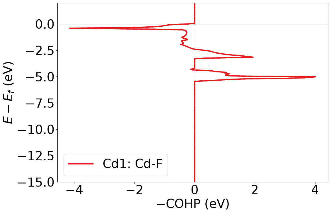
# Initialize the Description object
describe = Description(analysis_object=analyse)
describe.write_description()
The compound CdF2 has 1 symmetry-independent cation(s) with relevant cation-anion interactions: Cd1.
Cd1 has a cubic (CN=8) coordination environment. It has 8 Cd-F (mean ICOHP: -0.62 eV, 26.944 percent antibonding interaction below EFermi) bonds.
In the 8 Cd-F bonds, relative to the summed ICOHPs, the maximum bonding contribution is from the Cd(4d)-F(2p) orbital, contributing 35.0 percent, whereas the maximum antibonding contribution is from the Cd(4d)-F(2p) orbital, contributing 77.0 percent.
# Automatic interactive plots
fig = describe.plot_interactive_cohps(orbital_resolved=True, ylim=[-15,5], hide=True)
fig.show(renderer='notebook')
Due to sphinx rendering limitations for Plotly figures, the output is not directly visible within the notebook; please use the link to see the interactive orbital resolved plot
Get LOBSTER calculation quality and description#
This utility provides a quick overview of your LOBSTER calculation quality by reading the charge spilling and band overlaps file (if these are generated during LOBSTER runs). Optionally, one can obtain atom charge classification comparisons with the BVA method and a comparison between DOS from LOBSTER and VASP.
Note
The DOS comparisons and basis set utilized analysis are now limited to VASP calculations only. Support for other code output will be added in the future.
#### Change directory to your Lobster computations (Change this cell block type to Code and remove formatting when executing locally)
directory = Path("LobsterPy") / "tests" / "test_data" / "K3Sb"
# Get calculation quality summary dict
calc_quality_K3Sb = Analysis.get_lobster_calc_quality_summary(
            path_to_poscar=directory / "CONTCAR.gz",
            path_to_charge=directory / "CHARGE.lobster.gz",
            path_to_lobsterin=directory / "lobsterin.gz",
            path_to_lobsterout=directory / "lobsterout.gz",
            potcar_symbols=["K_sv", "Sb"], # if POTCAR exists, then provide path_to_potcar and set this to None
            path_to_bandoverlaps=directory / "bandOverlaps.lobster.gz",
            dos_comparison=True, # set to false to disable DOS comparisons
            bva_comp=True, # set to false to disable LOBSTER charge classification comparisons with BVA method
            path_to_doscar=directory / "DOSCAR.LSO.lobster.gz",
            e_range=[-20, 0],
            path_to_vasprun=directory / "vasprun.xml.gz",
            n_bins=256,
        )
calc_quality_K3Sb
{'minimal_basis': True,
 'charge_spilling': {'abs_charge_spilling': 0.83, 'abs_total_spilling': 6.36},
 'band_overlaps_analysis': {'file_exists': True,
  'limit_maxDeviation': 0.1,
  'has_good_quality_maxDeviation': True,
  'max_deviation': 0.0583,
  'percent_kpoints_abv_limit': 0.0},
 'charge_comparisons': {'bva_mulliken_agree': True, 'bva_loewdin_agree': True},
 'dos_comparisons': {'tanimoto_orb_s': np.float64(0.8532),
  'tanimoto_orb_p': np.float64(0.9481),
  'tanimoto_summed': np.float64(0.9275),
  'e_range': [-20, 0],
  'n_bins': 256}}
# Get a text description from calculation quality summary dictionary
calc_quality_k3sb_des = Description.get_calc_quality_description(
            calc_quality_K3Sb
        )
Description.write_calc_quality_description(calc_quality_k3sb_des)
The LOBSTER calculation used minimal basis. The absolute and total charge spilling for the calculation is 0.83 and 6.36 %, respectively. The bandOverlaps.lobster file is generated during the LOBSTER run. This indicates that the projected wave function is not completely orthonormalized; however, the maximal deviation values observed compared to the identity matrix is below the threshold of 0.1. The atomic charge signs from Mulliken population analysis agree with the bond valence analysis. The atomic charge signs from Loewdin population analysis agree with the bond valence analysis. The Tanimoto index from DOS comparisons in the energy range between -20, 0 eV for s, p, summed orbitals are: 0.8532, 0.9481, 0.9275.
Using plotting utilities#
from matplotlib import style
from pymatgen.io.lobster import Doscar, Icohplist
from lobsterpy.featurize.core import FeaturizeIcoxxlist
from lobsterpy.plotting import BWDFPlotter, InteractiveCohpPlotter, IcohpDistancePlotter, PlainCohpPlotter, PlainDosPlotter, get_style_list
You can alter the appearance of the static plots using the style sheet that comes with LobsterPy or use any of the readily available matplotlib style sheets.
Plot COHPs / COBIS / COOPs from Analysis object#
The are_cobis/are_coops arg must be set to True in the plotter depending on the type of files you analyze or want to plot. Here, we will keep them false as we are plotting COHPs.
# Using PlainCohpPlotter to get static plots of relevant bonds from Analysis object

style.use(get_style_list()[0]) # Use the LobsterPy style sheet for the generated plots

cohp_plot_static = PlainCohpPlotter(are_cobis=False, are_coops=False)
for plot_label, label_list in analyse.get_site_bond_resolved_labels().items():
    cohp = analyse.chemenv.completecohp.get_summed_cohp_by_label_list(label_list=label_list)
    cohp_plot_static.add_cohp(plot_label, cohp)
cohp_plot_static.get_plot(ylim=[-15,2]);
Note
You can get plots from orbital resolved analysis only when orbital_resolved arg is set to True when initializing the Analysis object.
label_list
['40', '33', '63', '30', '60', '53', '29', '64']
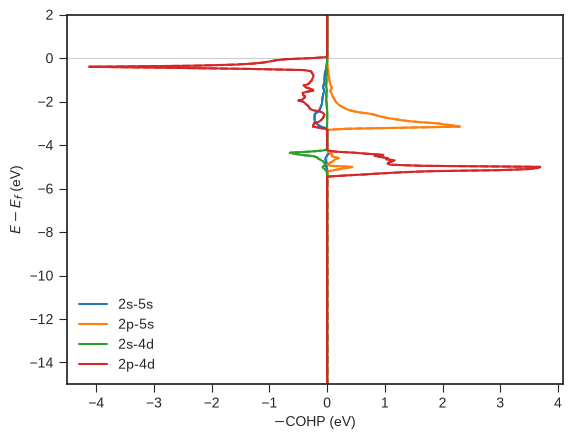
# Using PlainCohpPlotter to get static plots of relevant orbitals COHPs from Analysis object

style.use('default') # Complete reset the matplotlib figure style
style.use('seaborn-v0_8-ticks') # use one of the existing matplotlib style sheet

cohp_plot_static = PlainCohpPlotter()
for plot_label , orb_data in analyse.get_site_orbital_resolved_labels().items():
    for orb, plot_data in orb_data.items():
        mapped_bond_labels = [
                        item for item in plot_data["bond_labels"] for _ in range(len(plot_data["relevant_sub_orbitals"]))
                    ]
        cohp = analyse.chemenv.completecohp.get_summed_cohp_by_label_and_orbital_list(label_list=mapped_bond_labels,
                                                                                      orbital_list=plot_data["relevant_sub_orbitals"] *
                                                                                      len(plot_data["bond_labels"]))
        cohp_plot_static.add_cohp(orb, cohp)
cohp_plot_static.get_plot(ylim=[-15,2]);
# Using interactive plotter to add relevant cohps
interactive_cohp_plot = InteractiveCohpPlotter()
interactive_cohp_plot.add_all_relevant_cohps(analyse=analyse, label_resolved=False,orbital_resolved=True,suffix='')
fig = interactive_cohp_plot.get_plot()
fig.show(renderer='notebook')
Due to sphinx rendering limitations for Plotly figures, the output is not directly visible within the notebook; please use the link to see the interactive orbital resolved plot
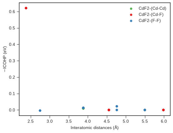
Plot ICOHPs / ICOBIS / ICOOPs Againsts bond-lengths#
#### Change directory to your Lobster computations (Change this cell block type to Code and remove formatting when executing locally)
directory = Path("LobsterPy") / "tests" / "test_data" / "CdF_comp_range"
# Plotting ICOHPs against distance

icohp_plotter = IcohpDistancePlotter(are_cobis=False, are_coops=False) # If reading and plotting ICOBIs or ICOOPs set args accordingly
icohplist = Icohplist(filename=directory / "ICOHPLIST.lobster.gz", are_cobis=False, are_coops=False)
icohp_plotter.add_icohps(label="CdF2", icohpcollection=icohplist.icohpcollection)

# color_interactions=False, will disable datapoints colouring based on atom pair types
icohp_plotter.get_plot(color_interactions=True, marker_size=20, alpha=0.9);
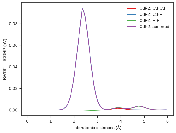
# Computing and Plotting BWDFs from ICOHPs

## We will use the featurizer to compute the BWDF
feat_icoxx = FeaturizeIcoxxlist(path_to_icoxxlist=directory / "ICOHPLIST.lobster.gz",
                               path_to_structure=directory / "CONTCAR.gz",
                               normalization="counts",
                               max_length=6,
                               min_length=0,
                               bin_width=0.1,
                               are_cobis=False,
                               are_coops=False)

bwdf = feat_icoxx.calc_bwdf() # this method will compute the BWDF for the entire structure and all unique atom pairs
# Plotting
bwdf_plotter = BWDFPlotter(are_cobis=False, are_coops=False) # If reading and plotting ICOBIs or ICOOPs set args accordingly
bwdf_plotter.add_bwdf(label="CdF2", bwdf=bwdf) # Add the BWDF data
bwdf_plotter.get_plot(sigma=0.3);
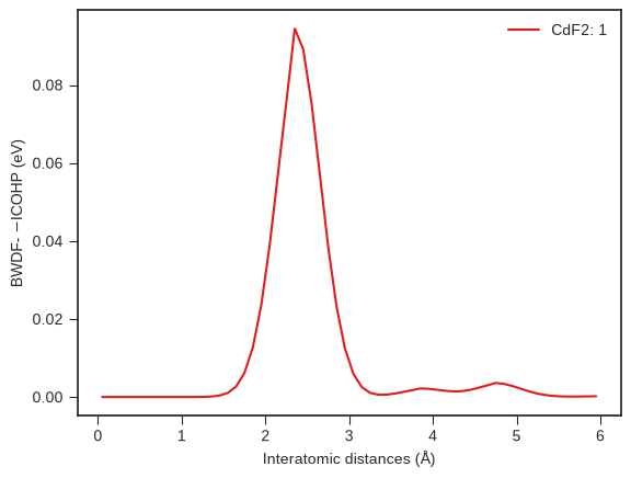
# One can also compute and plot BWDF for a single site of the structure
bwdf = feat_icoxx.calc_site_bwdf(site_index=1)

# Plotting
bwdf_plotter = BWDFPlotter(are_cobis=False, are_coops=False) # If reading and plotting ICOBIs or ICOOPs set args accordingly
bwdf_plotter.add_bwdf(label="CdF2", bwdf=bwdf) # Add the BWDF data
bwdf_plotter.get_plot(sigma=0.3);
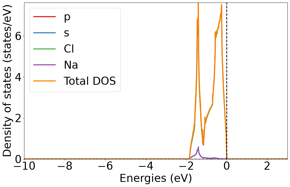
Plot DOS from Lobster#
# Load Lobster DOS (Change this cell block type to Code when executing locally)
directory = Path("LobsterPy") / "tests" / "test_data" / "NaCl_comp_range"
dos = Doscar(doscar=directory / 'DOSCAR.lobster.gz',
             structure_file=directory / 'CONTCAR.gz')
Plot total, element and spd dos
style.use('default') # Complete reset the matplotlib figure style
style.use(get_style_list()[0]) # Use the LobsterPy style sheet for the generated plots

dos_plotter = PlainDosPlotter(summed=True, stack=False, sigma=None)
dos_plotter.add_dos(dos=dos.completedos, label='Total DOS')
dos_plotter.add_dos_dict(dos_dict=dos.completedos.get_element_dos()) # Add element dos
dos_plotter.add_dos_dict(dos_dict=dos.completedos.get_spd_dos()) # add spd dos
dos_plotter.get_plot(xlim=[-10, 3]);
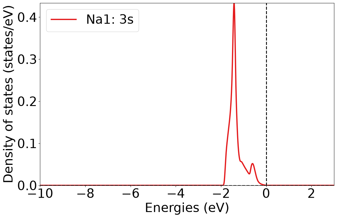
Plotting DOS at particular site and orbital
dos_plotter = PlainDosPlotter(summed=True, stack=False, sigma=0.03)
dos_plotter.add_site_orbital_dos(dos = dos.completedos, site_index=0, orbital='3s')
dos_plotter.get_plot(xlim=[-10, 3]);
Generate structure graph objects with LOBSTER data#
from lobsterpy.structuregraph.graph import LobsterGraph
Below code snippet will generate a networkx graph object with ICOHP, ICOOP, and ICOBI data as edge properties and charges as node properties.
#### (Change this cell block type to Code or copy it from here when executing locally)
graph_NaCl_all = LobsterGraph(
    path_to_poscar=directory / "CONTCAR.gz",
    path_to_charge=directory / "CHARGE.lobster.gz",
    path_to_cohpcar=directory / "COHPCAR.lobster.gz",
    path_to_icohplist=directory / "ICOHPLIST.lobster.gz",
    add_additional_data_sg=True,
    path_to_icooplist=directory / "ICOOPLIST.lobster.gz",
    path_to_icobilist=directory / "ICOBILIST.lobster.gz",
    path_to_madelung=directory / "MadelungEnergies.lobster.gz",
    which_bonds="all",
    start=None,
)
graph_NaCl_all.sg.graph.nodes.data() # view node data
NodeDataView({0: {'specie': 'Na', 'coords': array([0., 0., 0.]), 'properties': {'Mulliken Charges': 0.78, 'Loewdin Charges': 0.67, 'order_parameters': {'hexagonal planar': 8.492830879170379e-05, 'octahedral': 1.0, 'pentagonal pyramidal': 0.5000000000000001}, 'env': 'O:6'}}, 1: {'specie': 'Cl', 'coords': array([2.845847, 2.845847, 2.845847]), 'properties': {'Mulliken Charges': -0.78, 'Loewdin Charges': -0.67, 'order_parameters': {'hexagonal planar': 8.492830879170379e-05, 'octahedral': 1.0, 'pentagonal pyramidal': 0.5000000000000001}, 'env': 'O:6'}}})
graph_NaCl_all.sg.graph.edges.data() # view edge data
OutMultiEdgeDataView([(0, 1, {'to_jimage': (0, -1, -1), 'weight': 1, 'ICOHP': -0.56614, 'bond_length': 2.84585, 'bond_label': '30', 'ICOBI': 0.08482, 'ICOOP': 0.02824, 'ICOHP_bonding_perc': np.float64(1.0), 'ICOHP_antibonding_perc': np.float64(0.0)}), (0, 1, {'to_jimage': (-1, 0, -1), 'weight': 1, 'ICOHP': -0.56614, 'bond_length': 2.84585, 'bond_label': '28', 'ICOBI': 0.08482, 'ICOOP': 0.02824, 'ICOHP_bonding_perc': np.float64(1.0), 'ICOHP_antibonding_perc': np.float64(0.0)}), (0, 1, {'to_jimage': (-1, -1, 0), 'weight': 1, 'ICOHP': -0.56614, 'bond_length': 2.84585, 'bond_label': '24', 'ICOBI': 0.08482, 'ICOOP': 0.02824, 'ICOHP_bonding_perc': np.float64(1.0), 'ICOHP_antibonding_perc': np.float64(0.0)}), (0, 1, {'to_jimage': (0, 0, -1), 'weight': 1, 'ICOHP': -0.56616, 'bond_length': 2.84585, 'bond_label': '27', 'ICOBI': 0.08484, 'ICOOP': 0.02826, 'ICOHP_bonding_perc': np.float64(1.0), 'ICOHP_antibonding_perc': np.float64(0.0)}), (0, 1, {'to_jimage': (0, -1, 0), 'weight': 1, 'ICOHP': -0.5661700000000001, 'bond_length': 2.84585, 'bond_label': '23', 'ICOBI': 0.08484, 'ICOOP': 0.02826, 'ICOHP_bonding_perc': np.float64(1.0), 'ICOHP_antibonding_perc': np.float64(0.0)}), (0, 1, {'to_jimage': (-1, 0, 0), 'weight': 1, 'ICOHP': -0.5661700000000001, 'bond_length': 2.84585, 'bond_label': '21', 'ICOBI': 0.08484, 'ICOOP': 0.02826, 'ICOHP_bonding_perc': np.float64(1.0), 'ICOHP_antibonding_perc': np.float64(0.0)})])
Featurizer usage examples (Generates features from LOBSTER data for ML studies)#
Note
To use the batch featurizers, the path to the parent directory containing LOBSTER calculation outputs needs to be provided. For example, your directory structure needs to be like this:
parent_dir/lobster_calc_output_dir_for_compound_1/ parent_dir/lobster_calc_output_dir_for_compound_2/ parent_dir/lobster_calc_output_dir_for_compound_3/
the lobster_calc_output_dir_for_compound_* directory should contain all your LOBSTER outputs and POSCAR file.
In such a case path_to_lobster_calcs="parent_dir" needs to be set
from lobsterpy.featurize.batch import (BatchCoxxFingerprint, BatchIcoxxlistFeaturizer, BatchDosFeaturizer,
                                       BatchSummaryFeaturizer, BatchStructureGraphs)
BatchCoxxFingerprint#
BatchCoxxFingerprint provides a convenient way to directly generate fingerprint objects from COHP / COBI/ COOPCAR.lobster data. Generating fingerprints specifically for bonding, antibonding, and overall interactions is feasible.
One can also generate a pair-wise fingerprint similarity matrix dataframe (currently, only simple vector dot product or Tanimoto index are implemented)
## Initialize batch COXX featurizer (Change this cell block type to Code and remove formatting when executing locally)
fp_cohp_bonding = BatchCoxxFingerprint(
    path_to_lobster_calcs=directory / ".." / "Featurizer_test_data" / "Lobster_calcs",
    e_range=[-15, 0],
    feature_type="bonding",
    normalize=True, # affects only the fingerprint similarity matrix computation
    tanimoto=True, # affects only the fingerprint similarity matrix computation
    n_jobs=3,
    fingerprint_for='cohp' # changing this to cobi/coop will result in reading cobicar/coopcar file
)
# Access the fingerprints dataframe
fp_cohp_bonding.fingerprint_df
| COXX_FP | |
|---|---|
| mp-1000 | ([[-14.866071428571429, -14.598214285714286, -... |
| mp-2176 | ([[-14.866071428571429, -14.598214285714286, -... |
| mp-463 | ([[-14.866071428571429, -14.598214285714286, -... |
# Get the fingerprints similarity matrix
fp_cohp_bonding.get_similarity_matrix_df()
| mp-1000 | mp-2176 | mp-463 | |
|---|---|---|---|
| mp-1000 | 1.000000 | 0.001488 | 0.000036 |
| mp-2176 | 0.001488 | 1.000000 | 0.000000 |
| mp-463 | 0.000036 | 0.000000 | 1.000000 |
BatchIcoxxlistFeaturizer#
BatchIcoxxlistFeaturizer provides a convenient way to extract BWDF as features from the LOBSTER calculation directory. The extracted features consist of the following:
BWDF mean, standard deviation , skewness, kurtosis, weighted mean, and weighted standard deviation
Complete BWDF as columns in the dataframe
BWDF values sorted by bond distances as columns in the dataframe
Bond distances sorted by BWDF values as columns in the dataframe
# Initialize the batch ICOXXLIST featurizer
batch_icohp = BatchIcoxxlistFeaturizer(path_to_lobster_calcs=directory / ".." / "Featurizer_test_data" / "Lobster_calcs", # path to parent lobster calcs
            normalization="formula_units", # will normalize the BWDF values by formula units
            max_length=6, # maximum bond length for BWDF computation
            bin_width=0.1, # sets number for bins
            bwdf_df_type="stats", # Type of BWDF dataframe to generate (stats, binned, sorted_bwdf, sorted_dists)
            read_icobis=False, # set to true to read ICOBI data
            read_icoops=False, # set to true to read ICOOP data
            n_jobs=3,)
## Initialize batch ICOXXLIST featurizer (Change this cell block type to Code and remove formatting when executing locally)
batch_icohp = BatchIcoxxlistFeaturizer(path_to_lobster_calcs=directory / ".." / "Featurizer_test_data" / "Lobster_calcs", # path to parent lobster calcs
            normalization="formula_units", # will normalize the BWDF values by formula units
            max_length=6, # maximum bond length for BWDF computation
            bin_width=0.1, # sets number for bins
            bwdf_df_type="stats", # Type of BWDF dataframe to generate (stats, binned, sorted_bwdf, sorted_dists)
            read_icobis=False, # set to true to read ICOBI data
            read_icoops=False, # set to true to read ICOOP data
            n_jobs=3,)
# get the BWDF stats df
batch_icohp.get_bwdf_df()
Generating BWDF from ICOXXLIST: 0%| | 0/3 [00:00<?, ?it/s]
Generating BWDF from ICOXXLIST: 100%|██████████| 3/3 [00:00<00:00, 37.10it/s]
| pair_bwdf_sum_mean | pair_bwdf_mean_mean | pair_bwdf_std_mean | pair_bwdf_min_mean | pair_bwdf_max_mean | pair_bwdf_skew_mean | pair_bwdf_kurtosis_mean | pair_bwdf_sum_std | pair_bwdf_mean_std | pair_bwdf_std_std | ... | site_bwdf_kurtosis_std | bwdf_sum | bwdf_mean | bwdf_std | bwdf_min | bwdf_max | bwdf_skew | bwdf_kurtosis | bwdf_w_mean | bwdf_w_std | |
|---|---|---|---|---|---|---|---|---|---|---|---|---|---|---|---|---|---|---|---|---|---|
| mp-1000 | -2.38024 | -0.039671 | 0.304716 | -2.38024 | 0.0 | -7.550957 | 55.016949 | 2.177023 | 0.036284 | 0.278701 | ... | 9.351353 | -7.14072 | -0.119012 | 0.722113 | -5.39268 | 0.0 | -6.678922 | 44.843451 | -4.500476 | 1.567078 |
| mp-2176 | -3.123867 | -0.052064 | 0.398376 | -3.112027 | 0.0 | -7.55089 | 55.016285 | 3.882109 | 0.064702 | 0.494814 | ... | 1.525129 | -9.3716 | -0.156193 | 1.099228 | -8.56544 | 0.0 | -7.462189 | 54.087545 | -7.892133 | 2.195158 |
| mp-463 | -2.87552 | -0.047925 | 0.359435 | -2.80776 | 0.0 | -7.501752 | 54.497132 | 1.989998 | 0.033167 | 0.249226 | ... | 12.605783 | -8.62656 | -0.143776 | 0.762068 | -4.75344 | 0.0 | -5.333404 | 26.952803 | -4.183028 | 0.826071 |
3 rows × 37 columns
BatchDosFeaturizer#
BatchDosFeaturizer provides a convenient way to extract LOBSTER DOS moment features and fingerprints in the form of pandas dataframe from the LOBSTER calculation directory. The extracted features consist of the following:
Element and PDOS center, width, skewness, kurtosis, and edges
PDOS or total DOS fingerprint objects
## Initialize batch DOS featurizer (Change this cell block type to Code and remove formatting when executing locally)
batch_dos = BatchDosFeaturizer(path_to_lobster_calcs=directory / ".." / "Featurizer_test_data" / "Lobster_calcs", # path to parent lobster calcs
            use_lso_dos=True, # will enforce using DOSCAR.LSO.lobster
            add_element_dos_moments=True, # set to false to not have element moments dos features
            e_range=None, # setting this to none results in features computed for the entire energy range
            fingerprint_type="summed_pdos", # fingerprint type (s,p,d,f, summed_pdos)
            n_bins=256,
            n_jobs=3,)
# get the DOS moments df
batch_dos.get_df()
Generating PDOS moment features: 0%| | 0/3 [00:00<?, ?it/s]
Generating PDOS moment features: 33%|███▎ | 1/3 [00:00<00:00, 4.25it/s]
Generating PDOS moment features: 67%|██████▋ | 2/3 [00:00<00:00, 5.87it/s]
Generating PDOS moment features: 100%|██████████| 3/3 [00:00<00:00, 8.02it/s]
| s_band_center | s_band_width | s_band_skew | s_band_kurtosis | s_band_upperband_edge | Ba_s_band_center | Ba_s_band_width | Ba_s_band_skew | Ba_s_band_kurtosis | Ba_s_band_upperband_edge | ... | d_band_center | d_band_width | d_band_skew | d_band_kurtosis | d_band_upperband_edge | Zn_d_band_center | Zn_d_band_width | Zn_d_band_skew | Zn_d_band_kurtosis | Zn_d_band_upperband_edge | |
|---|---|---|---|---|---|---|---|---|---|---|---|---|---|---|---|---|---|---|---|---|---|
| mp-1000 | -11.2699 | 12.0711 | -0.2499 | 1.5351 | -27.0855 | -12.8945 | 14.2745 | 0.0684 | 1.0835 | -27.0855 | ... | NaN | NaN | NaN | NaN | NaN | NaN | NaN | NaN | NaN | NaN |
| mp-2176 | -5.2136 | 5.9110 | 0.3896 | 1.4512 | -10.4412 | NaN | NaN | NaN | NaN | NaN | ... | -6.5245 | 0.7822 | 4.602 | 50.478 | -6.5368 | -6.5245 | 0.7822 | 4.602 | 50.478 | -6.5368 |
| mp-463 | -12.2937 | 14.6993 | 0.5956 | 1.5582 | -26.1631 | NaN | NaN | NaN | NaN | NaN | ... | NaN | NaN | NaN | NaN | NaN | NaN | NaN | NaN | NaN | NaN |
3 rows × 65 columns
# get the DOS fingerprints df
batch_dos.get_fingerprints_df()
Generating DOS fingerprints: 0%| | 0/3 [00:00<?, ?it/s]
Generating DOS fingerprints: 33%|███▎ | 1/3 [00:00<00:00, 5.82it/s]
Generating DOS fingerprints: 67%|██████▋ | 2/3 [00:00<00:00, 7.69it/s]
Generating DOS fingerprints: 100%|██████████| 3/3 [00:00<00:00, 10.74it/s]
| DOS_FP | |
|---|---|
| mp-1000 | ([[-28.66463033203125, -28.524270996093747, -2... |
| mp-2176 | ([[-13.11592083984375, -12.971902519531252, -1... |
| mp-463 | ([[-28.161967734374997, -27.991663203125, -27.... |
BatchSummaryFeaturizer#
BatchSummaryFeaturizer provides a convenient way to extract summary stats as pandas dataframe from the LOBSTER calculation directory. The summary stats consist of the following:
ICOHP, bonding, antibonding percent (mean, min, max, standard deviation) of relevant bonds from LobsterPy analysis (Orbital-wise analysis stats data can also be included: Optional)
Weighted ICOHP ( ICOOP/ ICOBI: Optional)
COHP center, width, skewness, kurtosis, edge (COOP/ COBI: Optional)
Ionicity and Madelung energies for the structure based on Mulliken and Loewdin charges
## Initialize batch summary featurizer (Change this cell block type to Code and remove formatting when executing locally)
summary_features = BatchSummaryFeaturizer(
            path_to_lobster_calcs=directory / ".." / "Featurizer_test_data" / "Lobster_calcs",
            bonds="all",
            include_cobi_data=False,
            include_coop_data=False,
            e_range=[-15, 0],
            n_jobs=3,
        )
# get summary stats features
summary_features.get_df()
Generating LobsterPy summary stats: 0%| | 0/3 [00:00<?, ?it/s]
Generating LobsterPy summary stats: 33%|███▎ | 1/3 [00:06<00:12, 6.31s/it]
Generating LobsterPy summary stats: 67%|██████▋ | 2/3 [00:06<00:02, 2.83s/it]
Generating LobsterPy summary stats: 100%|██████████| 3/3 [00:08<00:00, 2.56s/it]
Generating LobsterPy summary stats: 100%|██████████| 3/3 [00:08<00:00, 2.98s/it]
Generating COHP/COOP/COBI summary stats: 0%| | 0/3 [00:00<?, ?it/s]
Generating COHP/COOP/COBI summary stats: 33%|███▎ | 1/3 [00:04<00:08, 4.02s/it]
Generating COHP/COOP/COBI summary stats: 67%|██████▋ | 2/3 [00:07<00:03, 3.72s/it]
Generating COHP/COOP/COBI summary stats: 100%|██████████| 3/3 [00:07<00:00, 2.53s/it]
Generating charge based features: 0%| | 0/3 [00:00<?, ?it/s]
Generating charge based features: 33%|███▎ | 1/3 [00:01<00:02, 1.25s/it]
Generating charge based features: 67%|██████▋ | 2/3 [00:01<00:00, 1.24it/s]
Generating charge based features: 100%|██████████| 3/3 [00:01<00:00, 1.67it/s]
| ICOHP_mean_avg | ICOHP_mean_max | ICOHP_mean_min | ICOHP_mean_std | ICOHP_sum_avg | ICOHP_sum_max | ICOHP_sum_min | ICOHP_sum_std | bonding_perc_avg | bonding_perc_max | ... | Mulliken_mean | Mulliken_min | Mulliken_max | Mulliken_std | Ionicity_Mull | Loewdin_mean | Loewdin_min | Loewdin_max | Loewdin_std | Ionicity_Loew | |
|---|---|---|---|---|---|---|---|---|---|---|---|---|---|---|---|---|---|---|---|---|---|
| mp-1000 | -0.340000 | -0.12 | -0.45 | 0.155563 | -2.273333 | -1.42 | -2.70 | 0.603398 | 0.782397 | 0.78970 | ... | 0.0 | -1.58 | 1.58 | 1.58 | 0.79 | 0.0 | -1.49 | 1.49 | 1.49 | 0.745 |
| mp-2176 | -1.070000 | -1.07 | -1.07 | 0.000000 | -4.280000 | -4.28 | -4.28 | 0.000000 | 0.853140 | 0.85314 | ... | 0.0 | -1.06 | 1.06 | 1.06 | 0.53 | 0.0 | -1.08 | 1.08 | 1.08 | 0.540 |
| mp-463 | -0.363333 | -0.29 | -0.40 | 0.051854 | -2.760000 | -2.38 | -3.52 | 0.537401 | 0.905510 | 0.91315 | ... | 0.0 | -0.81 | 0.81 | 0.81 | 0.81 | 0.0 | -0.82 | 0.82 | 0.82 | 0.820 |
3 rows × 37 columns
BatchStructureGraphs#
BatchStructureGraphs provides a convenient way to generate structure graph objects with LOBSTER data in the form of pandas dataframe from a set of the LOBSTER calculation directories.
## Initialize batch structure graphs featurizer (Change this cell block type to Code and remove formatting when executing locally)
batch_sg = BatchStructureGraphs(path_to_lobster_calcs=directory / ".." / "Featurizer_test_data" / "Lobster_calcs",
                                add_additional_data_sg=True,
                                which_bonds='all',
                                n_jobs=3,
                                start=None)
# get the structure graphs df
batch_sg.get_df()
Generating Structure Graphs: 0%| | 0/3 [00:00<?, ?it/s]
Generating Structure Graphs: 33%|███▎ | 1/3 [00:06<00:12, 6.11s/it]
Generating Structure Graphs: 67%|██████▋ | 2/3 [00:06<00:02, 2.78s/it]
Generating Structure Graphs: 100%|██████████| 3/3 [00:08<00:00, 2.56s/it]
Generating Structure Graphs: 100%|██████████| 3/3 [00:08<00:00, 2.95s/it]
| structure_graph | |
|---|---|
| mp-1000 | Structure Graph\nStructure: \nFull Formula (Ba... |
| mp-2176 | Structure Graph\nStructure: \nFull Formula (Zn... |
| mp-463 | Structure Graph\nStructure: \nFull Formula (K1... |