Command line interface#
Creating input files#
Note
Currently, the input set generated via pymatgen only supports PBE_54 standard POTCARS for identifying available basis sets for elements and adapting INCAR NBANDS.
Important tags in INCAR of VASP to pay attention to before performing lobster runs are NBANDS, NSW, and ISYM. A VASP static run must be performed (no movements of atoms, NSW = 0) before running the LOBSTER program. LOBSTER can only deal with VASP WAVECAR that contains results for the entire mesh or only half of it.
To do this, in the INCAR set, ISYM = -1 (complete mesh/symmetry switched off) or ISYM = 0 (half mesh/time-reversal). And to make sure WAVECAR is written, set LWAVE = .TRUE. For pCOHP analyses, one needs to have as many bands as there are orbitals on a local basis.
For pCOHP analyses using LOBSTER, however, you need to set NBANDS in the INCAR file manually.
With LobsterPy, these intricate details are handled with a single command. We need the standard VASP input files, i.e.
INCAR, KPOINTS, POTCAR and CONTCAR in the calculation directory. Once you have these files, one needs to run the following command:
lobsterpy create-inputs
The above command will create input files (INCAR and lobsterin) depending on the basis sets available in Lobster.
The NBANDS, NSW, and ISYM tags will be changed in the existing INCAR file, and new INCAR files will be written in the current directory.
The newly created INCAR file will be named INCAR.lobsterpy by default.
Simultaneously, lobsterin.lobsterpy files are created that are necessary for a lobster run (this is the file that instructs the LOBSTER program what computations must be performed).
You can also change the names of output files and path where they are saved using following optional tags:
lobsterpy create-inputs --file-incar-out <path/to/incar>/INCAR --file-lobsterin <path/to/lobsterin>/lobsterin
For example if Cd element has two basis sets 4d 5s 4d 5s 5p, thus following files are created:
INCAR.lobsterpy-0
INCAR.lobsterpy-1
lobsterin.lobsterpy-0
lobsterin.lobsterpy-1
The suffix “-0” & “-1” indicate input files corresponding to smaller and larger basis of Cd respectively.
Warning
The ‘KPOINTS’ file is not adapted; the user must select the appropriate grid density before starting VASP computations. Usually, a factor of 50 x crystallographic reciprocal lattice vectors (i.e., no factor of 2 * pi) is sufficient for reliable bonding analysis results.
Running VASP and Lobster program#
Before we start computations, it is important to organize the files in separate directories to avoid overwriting our results. So Let’s create two new directories named Basis_0 and Basis_1.
Copy ‘INCAR.lobsterpy-0, KPOINTS, POSCAR, POTCAR, lobsterin.lobsterpy-0’ files to Basis_0
Copy ‘INCAR.lobsterpy-1, KPOINTS, POSCAR, POTCAR, lobsterin.lobsterpy-1’ files to Basis_1
Rename ‘INCAR.lobsterpy-*’ to ‘INCAR’ and ‘lobsterin.lobsterpy-*’ to lobsterin in both the directories (* denotes 0 or 1)
Run VASP using the job submission script to your job scheduler on HPC .Eg:
sbatch submit.shWait for VASP computation to be finished.(Lobster program needs WAVECAR generated by VASP)
Now run the lobster program.
The sample job scripts for slurm job scheduler are provided below.
VASP job submission script
#!/bin/bash -l
#SBATCH -J vasp_job
#SBATCH --no-requeue
#SBATCH --export=NONE
#SBATCH --get-user-env
#SBATCH -D ./
#SBATCH --ntasks=144
#SBATCH --time=04:00:00
#SBATCH --partition=micro
#SBATCH --nodes=3
#SBATCH --output=vaspjob.out.%j
#SBATCH --error=vaspjob.err.%j

<path-to-vasp-bin>/vasp_std
Lobster job submission script
#!/bin/bash -l
#SBATCH -J lob_job
#SBATCH --no-requeue
#SBATCH --export=NONE
#SBATCH --get-user-env
#SBATCH -D ./
#SBATCH --ntasks=48
#SBATCH --time=04:00:00
#SBATCH --nodes=1
#SBATCH --output=lobsterjob.out.%j
#SBATCH --error=lobsterjob.err.%j

export OMP_NUM_THREADS=48

<path-to-lobster-bin>/lobster-4.1.0
Analyze the lobster outputs with automation#
Navigate to directory containing the files of lobster run and then one can use following commands:
1. Automatic analysis and plotting of COHPs/ICOHPs#
The
lobsterpy descriptioncommand will automatically analyze COHPs for relevant cation-anion bonds. This command also allows saving the output in a JSON file. Below is an example output of this command.
lobsterpy description --file-json description.json
The compound CdF2 has 1 symmetry-independent cation(s) with relevant cation-anion interactions: Cd1.
Cd1 has a cubic (CN=8) coordination environment. It has 8 Cd-F (mean ICOHP: -0.62 eV, 27.843 percent antibonding interaction below EFermi) bonds.
Following is the json file produced.
 {
   "formula": "CdF2",
   "max_considered_bond_length": 5.98538,
   "limit_icohp": [
     -100000,
     -0.1
   ],
   "number_of_considered_ions": 1,
   "sites": {
     "0": {
       "env": "C:8",
       "bonds": {
         "F": {
           "ICOHP_mean": "-0.62",
           "ICOHP_sum": "-4.97",
           "has_antibdg_states_below_Efermi": true,
           "number_of_bonds": 8,
           "bonding": {
             "integral": 7.93,
             "perc": 0.72157
           },
           "antibonding": {
             "integral": 3.06,
             "perc": 0.27843
           }
         }
       },
       "ion": "Cd",
       "charge": 1.57,
       "relevant_bonds": [
         "29",
         "30",
         "33",
         "40",
         "53",
         "60",
         "63",
         "64"
       ]
     }
   },
   "type_charges": "Mulliken"
}
lobsterpy description-quality --potcar-symbols "Na_pv Cl" --bvacomp --doscompcommand will automatically analyze your lobster calculation quality.
Note
The LOBSTER calculation directory need to have POTCAR, structure file (preferably CONTCAR), LOBSTER calculation input and output files to run the lobsterpy description-quality command successfully. If POTCAR is not available then you need to supply –potcar-symbols along with the command. Other optional files are vasprun.xml if –doscomp is switched on.
lobsterpy description-quality --potcar-symbols "Na_pv Cl" --bvacomp --doscomp --file-calc-quality-json calc_quality_description.json
The LOBSTER calculation used minimal basis. The absolute and total charge spilling for the calculation is 0.3 and 5.58 %, respectively. The projected wave function is completely orthonormalized as no
bandOverlaps.lobster file is generated during the LOBSTER run. The atomic charge signs from Mulliken population analysis agree with the bond valence analysis. The atomic charge signs from Loewdin
population analysis agree with the bond valence analysis. The Tanimoto index from DOS comparisons in the energy range between -5, 0 eV for s, p, summed orbitals are: 0.9785, 0.9973, 0.9953.
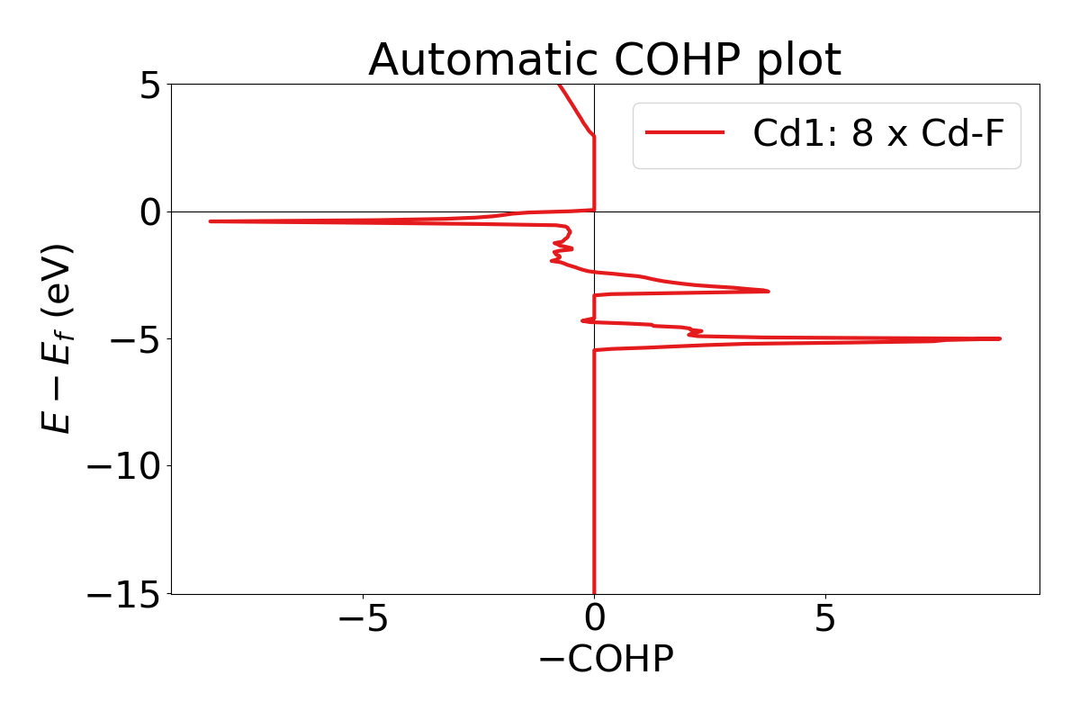
lobsterpy automatic-plotcommand will plot the results automatically. It will evaluate all COHPs with ICOHP values down to 10% of the strongest ICOHP. You can enforce an analysis of all bonds by usinglobsterpy automatic-plot --allbonds. Currently, the computed Mulliken charges will be used to determine cations and anions. If no CHARGE.lobster is available, the algorithm will fall back to the BondValence analysis from pymatgen. Please be aware that LobsterPy can only analyze bonds that have been included in the initial Lobster computation. Below is an example and sample output using this command.
lobsterpy automatic-plot --title 'Automatic COHP plot' --save-plot COHP.png
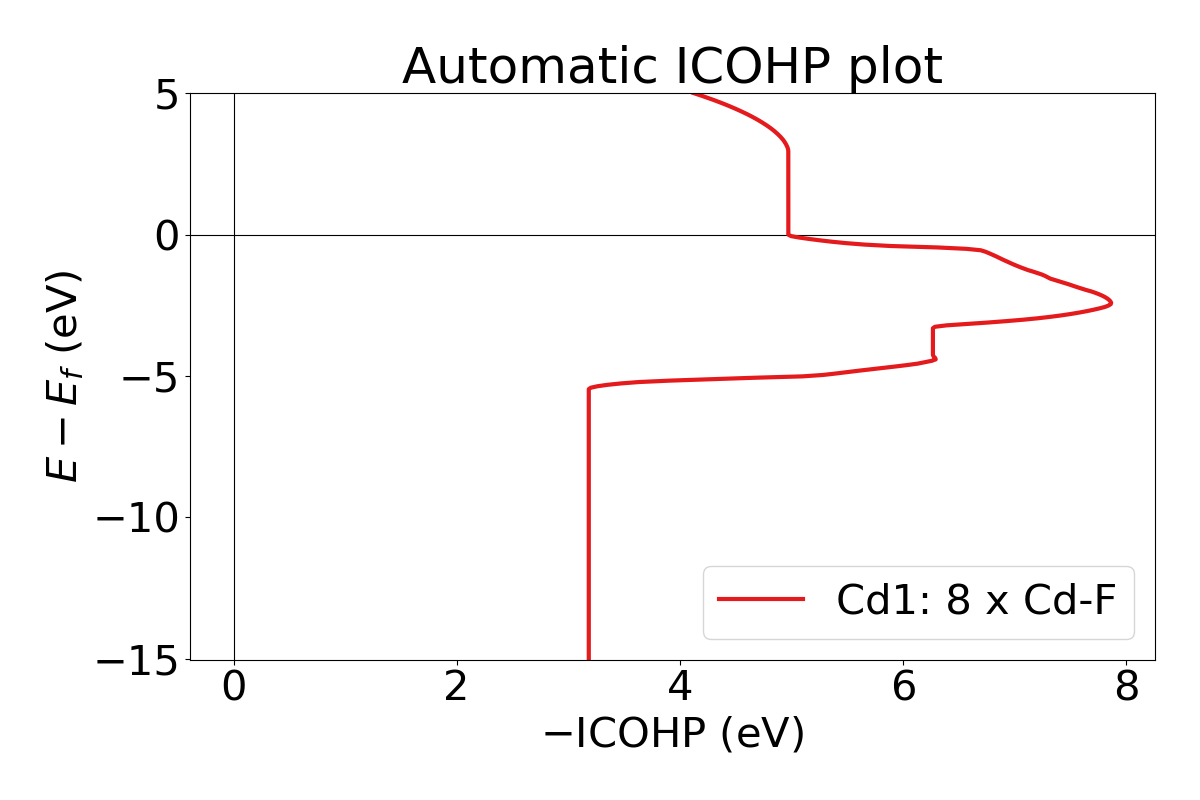
You can also plot integrated ICOHP computed by lobster by turning on
--integrated flag when executing lobsterpy automatic-plot
command. Below is an example and sample output using this command.
lobsterpy automatic-plot --title 'Automatic ICOHP plot' --integrated --save-plot ICOHP.png
lobsterpy automatic-plot-iacommand can be used to obtain a interactive plot of analysis automatically. It will evaluate all COHPs with ICOHP values down to 10% of the strongest ICOHP. You can enforce an analysis of all bonds by usinglobsterpy automatic-plot-ia --allbonds. Currently, the computed Mulliken charges will be used to determine cations and anions. If no CHARGE.lobster is available, the algorithm will fall back to the BondValence analysis from pymatgen. Please be aware that LobsterPy can only analyze bonds that have been included in the initial Lobster computation. You can also obtain a label resolved plot for all bonds using thelobsterpy automatic-plot-ia --allbonds --label-resolvedcommand. Below is an sample output usinglobsterpy automatic-plot-ia --label-resolvedcommand.
lobsterpy plot-auto-ia --save-plot-json auto_plot_data.jsoncan be used to save underlying plot data from the automatic analysis as a json file. This json file can be then loaded using monty package viamonty.serialization.loadfnfunction.
Note that --save-plot-json also works in combination with lobsterpy plot-auto subcommand.
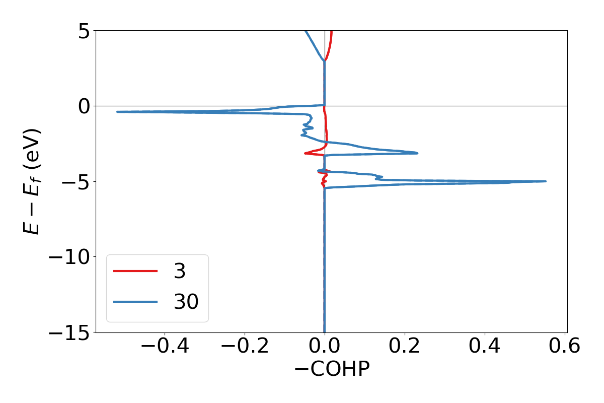
2. Plotting of COHPs/COBIs/COOPs#
You can plot COHPs/COBIs/COOPs from the command line.
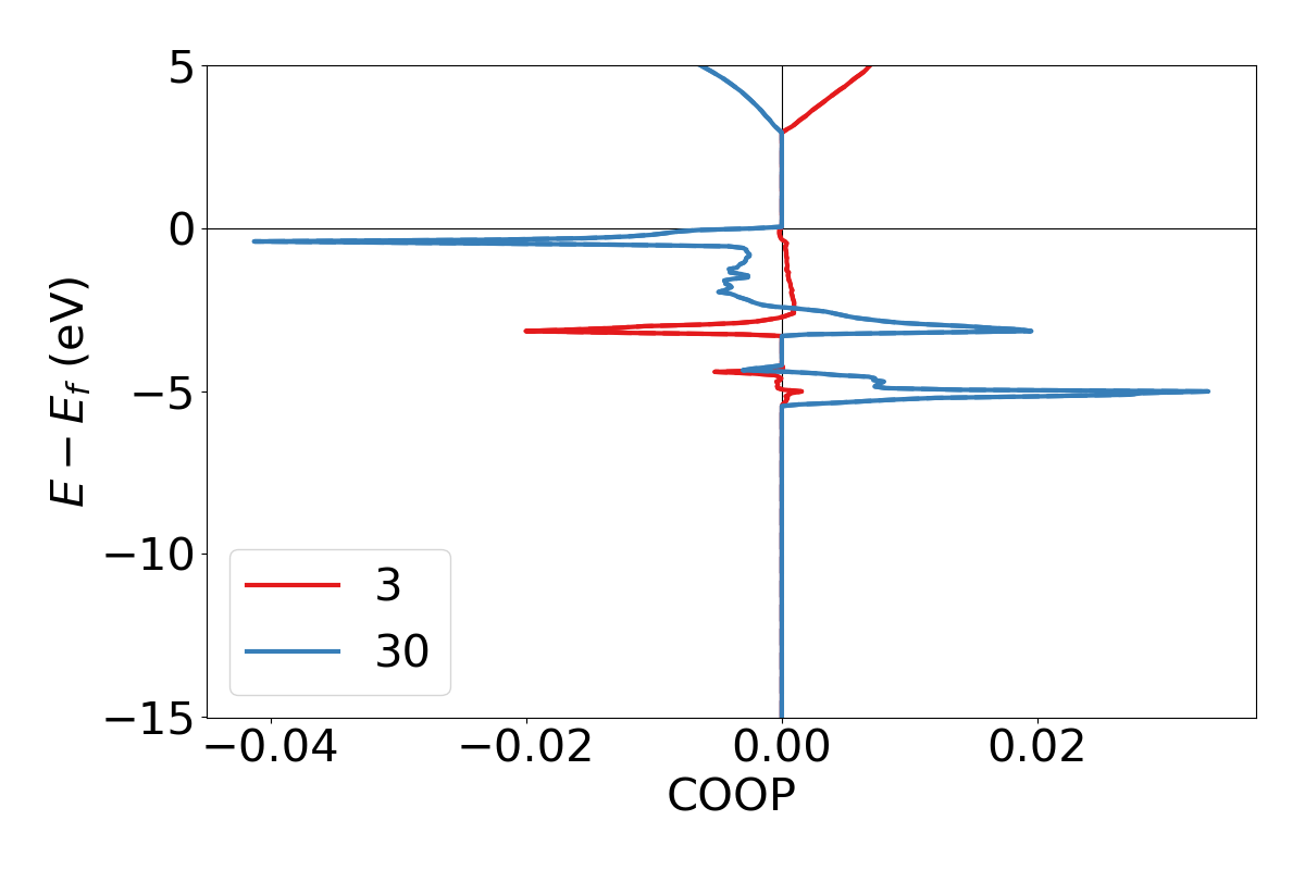
lobsterpy plot 3 30 will plot COHPs of the first and second bond from COHPCAR.lobster. It is possible to sum or integrate the COHPs as well (–summed, –integrated). You can switch to COBIs or COOPs by using –cobis or –coops, respectively. Below is an example output of command to plot COHP and COOP for bond labels 3 and 30.
lobsterpy plot 3 30 --save-plot COHP_330.png
lobsterpy plot 3 30 --coops --save-plot COOP_330.png
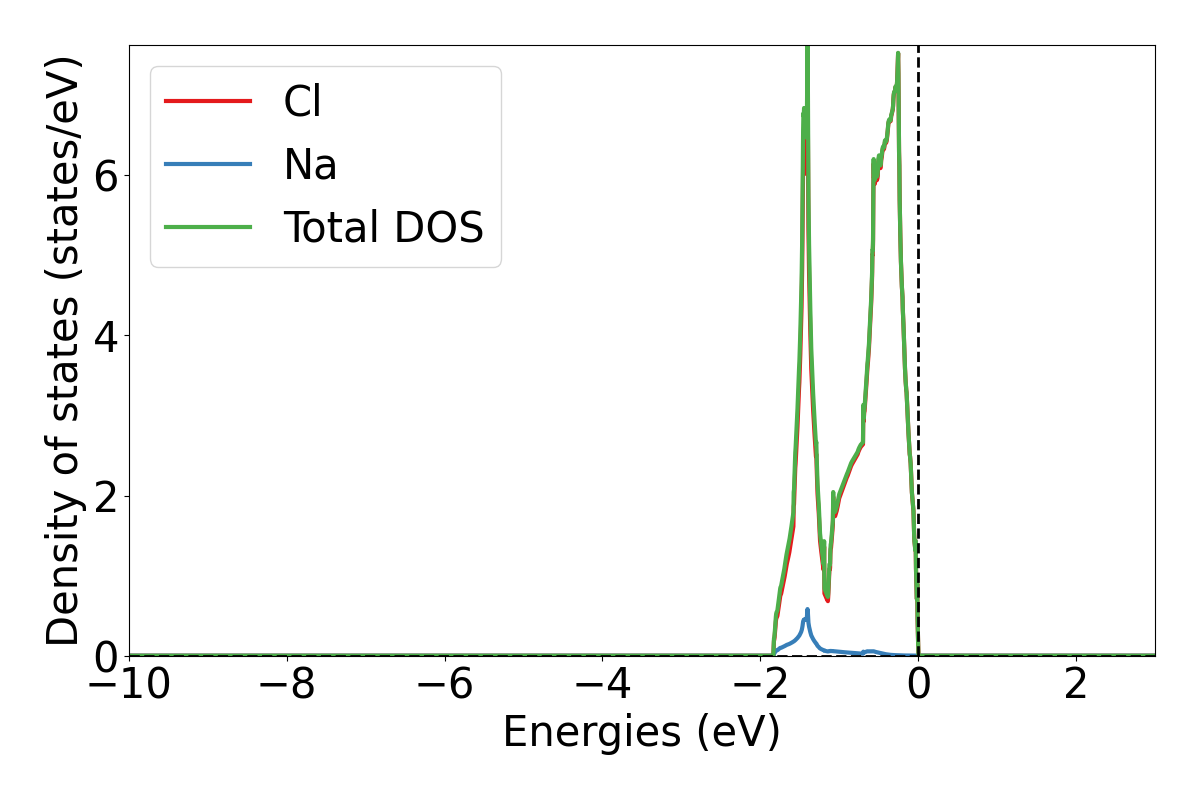
3. Plotting of DOS#
lobsterpy plot-dos --summedspinswill plot total and element DOS. Example output plot is shown below.
lobsterpy plot-dos --summedspins
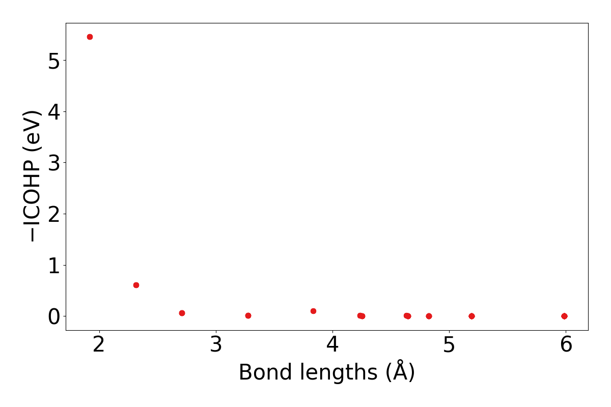
4. Plotting of ICOHPs/ ICOOPs/ICOBIS againsts bond lengths#
lobsterpy plot-icohps-distanceswill plot ICOHPs against bond lengths. Example output plot is shown below.
lobsterpy plot-icohp-distance
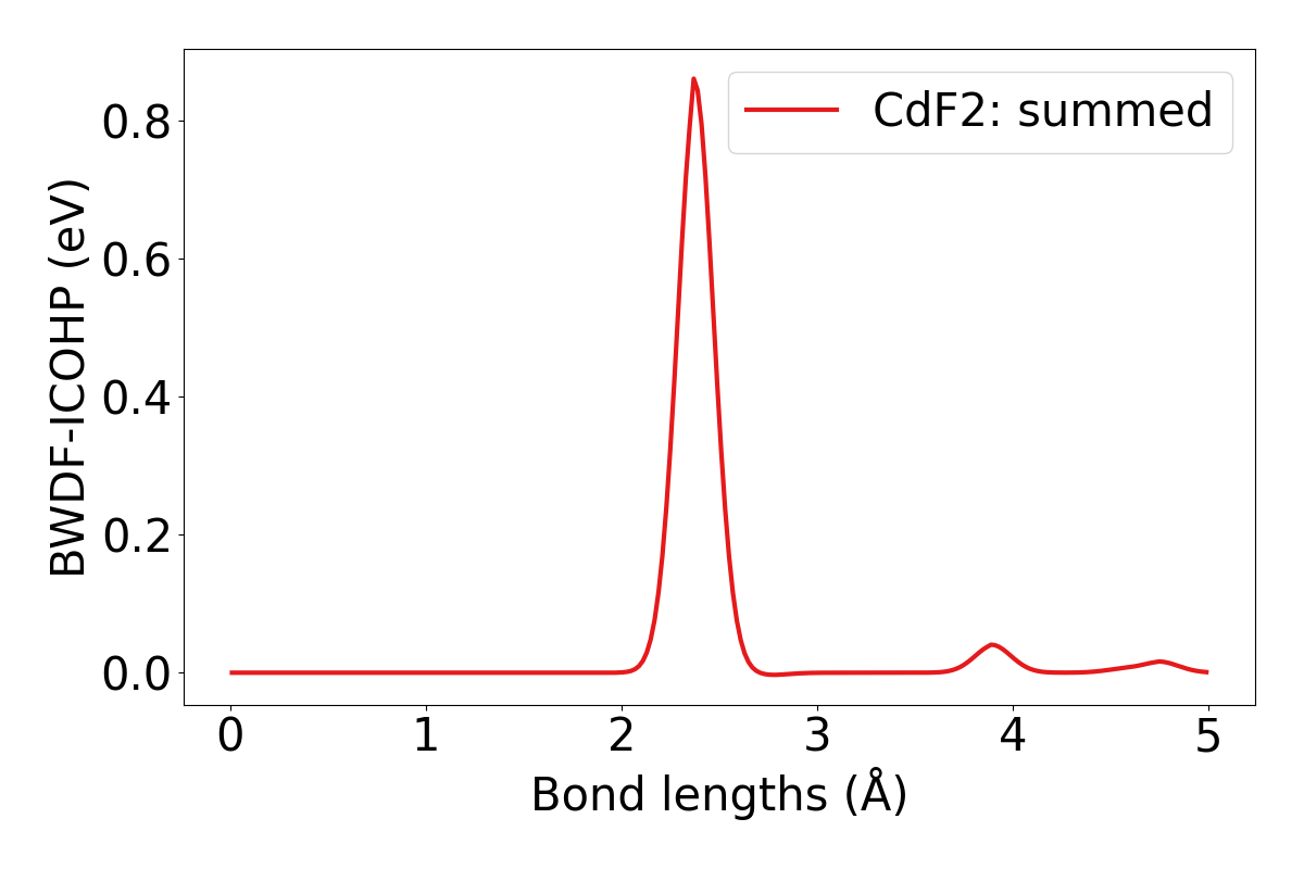
lobsterpy plot-bwdfwill plot Bond Weighted Distribution function (BWDF) using ICOHPs, ICOOPs or ICOBIs as weights against bond lengths. Example output plot is shown below. For more details on BWDFs check the orignal publication : https://doi.org/10.1002/anie.201404223
lobsterpy plot-bwdf --plot-negative --sigma 0.15
5. Additional Options#
You can also customize the style and parameters of the plots generated by using optional tags. One can easily get an overview of these using either of these commands:
lobsterpy automatic-plot --help
lobsterpy automatic-plot-ia --help
lobsterpy create-inputs --help
lobsterpy description --help
lobsterpy description-quality --help
lobsterpy plot-bwdf --help
lobsterpy plot-dos --help
lobsterpy plot-icohp-distance --help
lobsterpy plot --help